mptcptrace demo, experiment five
This is the fifth post of a series of five. Context is presented in the first post. The second post is here. The third post is here. The fourth post is here.
Fifth experiment
| Green at 0s: |
|
|---|---|
| Green at 5s: |
|
| Green at 15s: |
|
| Red: |
|
| Client: |
|
Last experiment of this series, we come back to the third experiment, and instead of adding a 1% loss rate after 15 seconds of the red subflow, we change the MPTCP scheduler and we use the round robin. It is worth to note that the round robin scheduler still respects the congestion window of the subflows.
Let’s see the evolution of the sequence number :
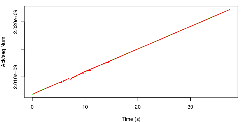
The first thing that we can see are the small steps between 5 and 15 seconds. We also have the impression that we use more the red subflow but if we zoom :

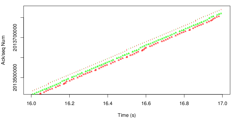
we can confirm that we use both subflows. We see 3 lines:
- The segments, because they are sent together at the sender, red and green subflows do not form two separate lines
- The green acks : we can see that they are closer to the segment line
- The red acks : we can see that all red acks are late from the MPTCP point of view. This is normal since the green delay is shorter.
If we look at the evolution of the sequence number between 5 and 15 seconds, we can observe a series of stairs.

If we take a close at one of the this stairs :
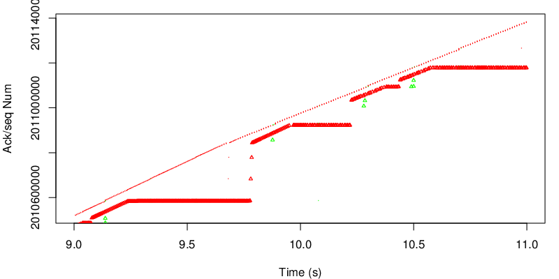
because the green subflow is lossy during this period, we have reordering. Because we use the round robin scheduler, MPTCP still decides to send some data over the green path.
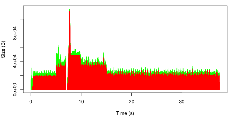
If we now take a look at the evolution of the goodput :
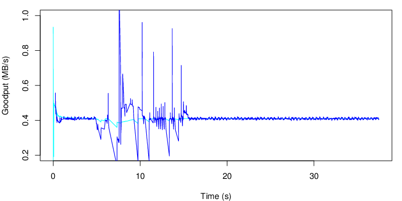
We can see the perturbation of the lossy link over the “instantaneous” goodput.
However the impact on the average goodput is somehow mitigated. Depending of the application, these variations may be problematic or not.
If we take a look at the evolution of the MPTCP unacked data, we see a lot of variations during the period 5 to 15 seconds. This is due to the reordering that happens during this period. This is not a big issue as long as the receive window is big enough to absorb these variations. In some scenarios this may be an issue if the window is too small. We may also remark that MPTCP may use more memory in this case on the receiver due to the buffer auto-tuning.
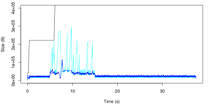
Finally, we can take a look at the evolution of the unacked data at the TCP level.
We can observe that we use both subflows during the whole connection but losses between 5 and 15 seconds on the green subflow leads to a bigger usage of the red subflow during this period.
Conclusion
This ends the series of posts that shows some basic MPTCP experiments. mptcptrace has been used to get the values out of the traces and R scripts have been used to produce the graphs. However we did not really post process the data in R. We have more experiments and visualizations that we will present later.